
Blockchain And Cryptocurrencies:
A Data Science Tutorial
By Julian Castrence
December 2019
Introduction
On January 3rd, 2009, Satoshi Nakamoto mined the Bitcoin genensis block, the first ever block to join (or more appropriately, create) Bitcoin's blockchain, and thus the world's first decentralized cryptocurrency was born. Satoshi Nakamoto would continue to be the sole miner of Bitcoin blocks for the next several months and would accumulate a holding of 1 million BTC. In 2009 however, no one knew what a Bitcoin was. No one knew about cryptocurrencies or the blockchain. The price of a single Bitcoin was approximately a thousandth of a penny. For the next two years, the Bitcoin protocol would slowly gain more traction from crypto enthusiasts, dark web users, investors, and skeptics, but at under the price of a single US dollar, Bitcoin had not gained any real attention from the general public.
Fast forward to over a decade later and a single Bitcoin is worth over 7000 USD. At it's peak in December 2017, Bitcoin was almost at 20,000 USD. Hundreds of other cryptocurrencies have followed in stride and the current total market capitalization of the crypto market today is 190 billion USD. Internet money that was once thought to be worth nothing more than a couple of pennies is being used across the world to transfer real monetary capital every day. What's more is that the revolutionary and powerful technology behind cryptocurrencies, blockchain, is being leveraged and applied to an ever-increasing list of fields.
The purpose of this tutorial is to tour the reader through the data science life cycle, using Python3 as a vehicle, while also educating them on the cryptocurrency market and blockchain technology. To begin, we will scrape Bitcoin data and collect the appropriate files from the internet to obtain a large collection of data on cryptocurrencies and their respective blockchains. Then, we will process this data into dataframes, converting our raw data into a more digestable form. Next, we'll analyze our data using data visualization techniques and explore the Bitcoin bubbles, the top cryptocurrencies of today, and trading technical analysis. Finally, we'll use our analysis to predict Bitcoin prices through machine learning and use our results to draw insight about cryptocurrencies. The hope is that the reader walks away with a better understanding of the applications of data science and a newfound interest in blockchain technology. </p>
Collecting The Data
Libraries
The following Python3 libraries are required for this tutorial. If you do not have html5lib or lxml installed natively, uncomment the respective !pip install commands. To read more about the libraries we will use:
datetime, numpy, pandas, requests, seaborn, beautifulsoup, matplotlib, scikit-learn
import datetime as dt
import numpy as np
import pandas as pd
import requests as req
import seaborn as sns
import warnings

from bs4 import BeautifulSoup as bs4
from matplotlib import pyplot as plt
from matplotlib.pyplot import figure
from pandas.plotting import register_matplotlib_converters
from scipy.stats import f
from sklearn import linear_model
from sklearn import model_selection
from sklearn.linear_model import LinearRegression

# !pip install html5lib
# !pip install lxml

warnings.filterwarnings('ignore')
Data Collection
The first step in the data science life cycle is to collect your data. For this project we will be gathering our data from several different sources. Coin Metrics is an execellent source for data on cryptocurrencies. Their database contains metrics on coin prices, market capitalization, mining difficulty, transaction data, and so much more. We will be using their free community data for the top 5 coins on the crypto market: Bitcoin (BTC), Ethereum (ETH), Ripple (XRP), Bitcoin Cash (BCH), and Litecoin (LTC). All csv files required to follow along are included on my GitHub, but for those who are interesed, the data for these coins and a lot more can be downloaded here. Once we have the csv files, we will turn them into dataframes with Pandas. This will allow us to better manipulate the data when it's time to analyze it.
# Data from https://coinmetrics.io/data-downloads/
# Turn each csv into a dataframe for each coin
btc = pd.read_csv('data/btc.csv')
eth = pd.read_csv('data/eth.csv')
xrp = pd.read_csv('data/xrp.csv')
bch = pd.read_csv('data/bch.csv')
ltc = pd.read_csv('data/ltc.csv')
The data we have so far is great, but it only includes the daily closing prices for each coin, which will be a little lacking for price analysis later. CoinMarketCap includes more in-depth data on coin prices, including daily highs, lows, and openings. They don't provide csv downloads but their front-end presents price data in a way that we can easily scrape it. Navigate to their historical data for Bitcoin prices and set the dates to All Time. Using the Requests library and BeautifulSoup, we can make a request to CoinMarketCap and scrape their web contents in the form of HTML. We can once more use BeautifulSoup to neatly pull the actual data out of the HTML, which is simply stored in a table tag. Again, this data has been saved to the GitHub repository and can be accessed from there alternatively.
# Data from "https://coinmarketcap.com/currencies/bitcoin/historical-data/?start=20130428&end=20191208"
# Send a request to CoinMarketCap
# r = req.get(coinmarketcap_url)

# Scrape the HTML using BeautifulSoup and store the contents of the <thead> and <tbody> tags since this is where the
# actual data is
# root = bs4(r.content, 'html.parser')
# thead = root.find('thead')
# tbody = root.find('tbody')

# Insert the <thead> and <tbody> tags into a <table> tag so that Pandas can recognize it then convert to a dataframe
# table = '<table>' + str(thead) + str(tbody) + '</table>'
# coinmarketcap = pd.read_html(str(table))[0]

# This data has been saved to a csv file in the event that the links no longer work

# Uncomment the following line to save your scraped data to a csv file:
# coinmarketcap.to_csv('coinmarketcap.csv', index=False)

# Uncomment the following line to get the data from the GitHub repo instead of scraping
coinmarketcap = pd.read_csv('data/coinmarketcap.csv')
We have a lot of technical data regarding the metrics of cryptocurrency blockchains and Bitcoin price data. Let's collect some non-technical data that may also prove useful in analyzing Bitcoin's price data later. Google Trends provides data on the search frequency of a given term. We'll download a csv containing the search popularity of the search term "Bitcoin" over time.
# Data from https://trends.google.com/trends/explore?date=2019-04-01%202019-11-30&geo=US&q=Bitcoin
# Turn the Google Trends data into a pandas dataframe
googletrends = pd.read_csv('data/multiTimeline.csv')
We now have all the data we need! Let's move on to data processing.
Processing The Data
Data Cleaning and Fixing
Now that we have all of our data, we need to process it. The first step is to clean and fix the data so that it is easier to manage. Let's start by taking a look at the Coin Metrics dataset.
btc.head()
eth.head()
xrp.head()
bch.head()
ltc.head()
There are several steps we need to take to tidy our Coin Metrics data. The first thing we need to do is reduce the amount of columns in each dataframe. Currently, each dataframe has around 30 to 40 columns and we most definitely won't be needing all of them. Coin Metrics provides a data dictionary that we can use to figure out what type of data each column represents. Let's sort through the columns and identify the metrics we actually care about.
- AdrActCnt - Total active addresses on the network per day
- BlkCnt - Total blocks mined / verified per day
- BlkSizeMeanByte - Mean block size (bytes) of total blocks mined / verified per day
- CapMrktCurUSD - Total market capitalization (USD) per day
- DiffMean - Mean difficulty (varies for coin) to mine / verify all new blocks per day
- PriceUSD - Closing price (USD) of 1 coin at 00:00 UTC per day
- TxCnt - Total transactions per day
- TxTfrValAdjUSD - Total value (USD) of all coin transfers per day
# Cleaning Coinmetrics

# Takes in a dataframe from Coin Metrics and returns a tidy dataframe
def clean_coinmetrics(df, is_bitcoin=False):
    # Check if we are cleaning BTC data
    if is_bitcoin:
        # Keep only columns that we care about and rename them
        df = df[['date', 'AdrActCnt', 'BlkCnt', 'BlkSizeMeanByte', 'CapMrktCurUSD', 'DiffMean', 'PriceUSD', \
                'TxCnt', 'TxTfrValAdjUSD']]
        df = df.rename(columns={'AdrActCnt':'activeAddresses', 'BlkCnt':'blockCount', \
                                'BlkSizeMeanByte':'meanBlockSize', 'CapMrktCurUSD':'marketCap', \
                                'DiffMean':'meanDifficulty', 'PriceUSD':'price', 'TxCnt':'txCount', \
                                'TxTfrValAdjUSD':'transferVolume'})
    else:
        # Keep only columns that we care about and rename them
        df = df[['date', 'AdrActCnt', 'BlkCnt', 'CapMrktCurUSD', 'PriceUSD', 'TxCnt', 'TxTfrValAdjUSD']]
        df = df.rename(columns={'AdrActCnt':'activeAddresses', 'BlkCnt':'blockCount', 'CapMrktCurUSD':'marketCap', \
                                'PriceUSD':'price', 'TxCnt':'txCount', 'TxTfrValAdjUSD':'transferVolume'})
    # Convert the dates column into datetime objects
    dates = []
    for i, row in df.iterrows():
        dates.append(dt.datetime.strptime(row['date'], '%Y-%m-%d').date())
    df['date'] = dates
    # Drop rows that are missing data and reset the index
    df = df.dropna()
    df = df.reset_index(drop=True)

    return df

# Bitcoin
btc = clean_coinmetrics(btc, is_bitcoin=True)

# Ethereum
eth = clean_coinmetrics(eth)

# Ripple
xrp = clean_coinmetrics(xrp)

# Bitcoin Cash
bch = clean_coinmetrics(bch)

# Litecoin
ltc = clean_coinmetrics(ltc)
btc.head()
eth.head()
Our Coin Metrics data is now tidy. Cleaning the rest of our data will follow a similar pattern. We'll change date strings to datetime objects, give columns more readable names, and get rid of any rows with missing data.
# Cleaning CoinMarketCap

# Turn date strings into datetime objects
coinmarketcap_dates = []
for i, row in coinmarketcap.iterrows():
    coinmarketcap_dates.append(dt.datetime.strptime(row['Date'], '%b %d, %Y').date())
coinmarketcap['Date'] = coinmarketcap_dates

# Give columns more readable names
coinmarketcap = coinmarketcap.rename(columns={'Date':'date', 'Open*':'open', 'High':'high', 'Low':'low', \
                                              'Close**':'close', 'Volume':'volume', 'Market Cap':'marketCap'})

# Sort dataframe so data is chronological and reset the indices
coinmarketcap = coinmarketcap.sort_values(by='date')
coinmarketcap = coinmarketcap.reset_index(drop=True)
coinmarketcap.head()
Identifying the columns from our CoinMarketCap data:
- open - Opening price (USD) of Bitcoin that day
- high - Highest price (USD) of Bitcoin that day
- low - Lowest price (USD) of Bitcoin that day
- close - Closing price (USD) of Bitcoin that day
- volume - Total volume (USD) of all Bitcoin movement on popular exchanges that day
- marketCap - Total market capitalization (USD) of all Bitcoin units that day
# Cleaning Google Trends

# Fix the the column headers by removing the first row and renaming columns
googletrends = googletrends.drop('Day')
googletrends = googletrends.reset_index()
googletrends = googletrends.rename(columns={'index':'date', 'Category: All categories':'searchPopularity'})

# Turn date strings into datetime objects and search popularity into int types
googletrends_dates = []
googletrends_search = []
for i, row in googletrends.iterrows():
    googletrends_dates.append(dt.datetime.strptime(row['date'], '%Y-%m-%d').date())
    googletrends_search.append(int(row['searchPopularity']))
googletrends['date'] = googletrends_dates
googletrends['searchPopularity'] = googletrends_search
googletrends.head()
Identifying the columns from our Google Trends data:
- searchPopularity - Taken directly from Google Trends:
"Numbers represent search interest relative to the highest point on the chart for the given region and time. A value of 100 is the peak popularity for the term. A value of 50 means that the term is half as popular. A score of 0 means there was not enough data for this term."
Now that our data is clean, digestible, and understandable, we can start to play with it. Let's do some data analysis!
Exploring The Data
Case Study 1: Breaking Down The Blockchain
But what actually is a blockchain? Let's try and understand how the technology behind cryptocurrencies work then strengthen our understanding by doing some data visualization.
Decentralization
To fully understand how blockchains work you first have to understand what problem they are solving. Let's pretend there are two people; Alice and Bob. Alice wants to pay Bob for mowing her lawn. Alice could send money from her bank account to Bob's bank account. But what if before Alice is able to send her money, hackers break into her bank account and steal all of her funds? What if Alice's bank doesn't like Bob's banks and charges expensive fees for transfers to Bob's bank? How can Alice even trust that the banks are doing a good job and making sure that everyone's account balance is accurate? If Alice and Bob are exchanging money using a fiat currency like the USD, what if the government just decides to print a lot of money and completely lower the value of Alice's worth? These are all possible scenarios because banks and fiat currencies are centralized, meaning they are controlled by some type of entity. Cryptocurrencies (for the most part) are decentralized, meaning that there is no one entity in control of everything. Effectively everyone, or the network, is in control, and because of this no one has to be trusted. This is possible through blockchain.Public Ledger
If there is no bank to keep track of my balance or no physical realization of monetary value like USD, how can we even have transactions? Cryptocurrencies like Bitcoin record transactions on a public ledger. Every single Bitcoin that has ever existed is recorded on the public ledger. In fact, Bitcoins are not even coins at all, they are simply transactions that have not yet been spent. For example, if Alice pays Bob 1 Bitcoin and this transaction is recorded on the public ledger for everyone to see, does Bob even need to keep track of a balance or hold onto a physical Bitcoin? As long as everyone recognizes on the public ledger that Bob was paid a valid Bitcoin from Alice, then as long Bob doesn't spend that Bitcoin, or post a transaction to the public ledger that he no longer owns the Bitcoin, then Bob still has one Bitcoin. But what's to stop Bob from telling Charlie that he paid him one Bitcoin, but not recording the transaction to the public ledger? What's to stop Alice from writing to the public ledger that Bob paid her back the Bitcoin right after she paid him? Where do Bitcoins even come from?Cryptographic Hash Functions
Think of a shredder that takes in a piece of paper and turns it into a pile of paper string. Would you be able to put it back together? What if you took a different piece of paper and put it through the shredder. It would come out to a completely different pile of paper string. A cryptographic hash function is simply a shredder that works with data.Blocks And The Blockchain
A block in it's most basic form is simply a list of transactions. Every Bitcoin transaction to ever occur is stored in a block. A block is then hashed with a cryptographic hash function to create a unique hash value and it stores this value. A blockchain is a string of blocks that requires each block to have the hash value of the block that came before it. This makes the blockchain immutable. Since a blockchain is simply a list of transactions that cannot be altered, it is a perfect vehicle for the public ledger. Blockchains are distributed, decentralized, public ledgers.Digital Signature
Without getting too technical, a digital signature is exactly what it sounds like, and exponentially more effective than a hand-written signature. A Bitcoin digital signature is essentially a number from 0 to 2 raised to the 256th power that is not revealed when signing a transaction. To put into perspective how hard it would be to attempt to guess someone's digital signature, watch this video. All Bitcoin transactions are signed and because of this, Alice cannot fake a transaction where Bob pays her back.Consensus
Without a form of consensus on how blocks should be added to the blockchain, everyone's public ledgers (copies of the blockchain) will look different, and nothing can stop Bob from sending a transaction to Charlie where he pays him one Bitcoin, then produces his own public ledger without this transaction. Consensus enforces what steps need to be taken to add a block to the blockchain. In the Bitcoin protocol, a block's hash value must be lower than a specific number. This makes it difficult to calculate valid block hashes and thus it cannot be done by one person. The consensus also dictates that only the longest blockchain should be valid. With consesus, Bob cannot send fake transactions that he later takes back (this is known as double spending).Mining
In Bitcoin, the process of enforcing consensus on a block of transactions is called mining. Bitcoin miners compete to find the next valid hash value so that they can add the next block to the blockchain. They do this because the person who adds the next block to the blockchain gets rewarded in Bitcoin. This is how new Bitcoin are introduced to the network. The fact that it was so hard to calculate the hash value of the next block is called "proof-of-work". If more miners join the network, then block hashes will be found quicker, and blocks will get added to the blockchain faster. To keep the proof-of-work from becoming easier to compute for the Bitcoin network over time, the difficulty, or range of allowed block hashes, is automatically scaled to the computing power of the network and constantly increases as miners join the network. This constant increase in difficulty is how the Bitcoin network maintains the proof-of-work.In Conclusion
This explanation of blockchain technology is not meant to be exhaustive by any means. Only the surface was scratched and many complex layers of this new technology were left out for the sake of time. The purpose of this walkthrough was to prepare the reader just enough for data analysis and also to spark an interest in blockchain. If you would like a more in-depth explanation of blockchains and how cryptocurrencies like Bitcoin work, I encourage you to watch this video.Let us now further improve our understanding of blockchains by analyzing at our Bitcoin data from Coin Metrics. We will plot each metric against the date to see how different aspects of the Bitcoin blockchain change over time.
# Plot each metric of Bitcoin against time

plt.figure(figsize=(20, 14))

# Price
plt.subplot(3, 3, 1)
plt.plot(btc.date, btc.price, 'r-')
plt.title("Price (USD)")
plt.ylabel("USD")

# Transaction Count
plt.subplot(3, 3, 2)
plt.plot(btc.date, btc.txCount, 'm-')
plt.title("Transaction Count (USD)")
plt.ylabel("USD")

# Transfer Volume
plt.subplot(3, 3, 3)
plt.plot(btc.date, btc.transferVolume, 'c-')
plt.title("Transfer Volume (USD)")
plt.ylabel("USD")

# Market Capitalization
plt.subplot(3, 3, 4)
plt.plot(btc.date, btc.marketCap, 'y-')
plt.title("Market Capitalization (USD)")
plt.ylabel("USD")

# Mean Difficulty
plt.subplot(3, 3, 6)
plt.plot(btc.date, btc.meanDifficulty, 'b-')
plt.title("Mean Difficulty")
plt.ylabel("Bitcoin Difficulty")

# Active Addresses
plt.subplot(3, 3, 7)
plt.plot(btc.date, btc.activeAddresses, 'g-')
plt.title("Active Addresses")
plt.ylabel("Addresses")

# Mean Block Size
plt.subplot(3, 3, 8)
plt.plot(btc.date, btc.meanBlockSize, '-', color='#ffa500')
plt.title("Mean Block Size")
plt.ylabel("Bytes")

# Block Count
plt.subplot(3, 3, 9)
plt.plot(btc.date, btc.blockCount, 'k-')
plt.title("Block Count")
plt.ylabel("Blocks");

The visualization of Bitcoin data plotted against time gives us some insight as to which metrics could be correlated. This will help us create our linear model. Price and market capitalization are very obviously strongly correlated. This can be explained since, as the price of a single Bitcoin goes up or down, the price change will have a scaled effect on the total market capitalization. Transaction count and number of active addresses are also very strongly related. Again, one could formulate that as more people join the network, there will inherently be more transactions as a result. At a glance, transaction volume looks like it would be strongly correlated with price, but further analysis would be required before any conclusions are made. As stated, the mean difficulty to hash each block continues to increase regardless of the fluctuations of other metrics as the network automatically scales to the number of nodes in the network. Only once does difficulty significantly change direction, during the bear market of 2018. As a result of the balance between difficulty and number of nodes on the network, the average number of blocks being added to the network stays fairly constant, hovering around 120 - 180 blocks a day, approximately 1 block every 10 minutes. Surprisingly the mean block size increases over time. This is slightly unexpected since Bitcoin blocks have an artificial limit of around 1 million bytes to limit the number of transactions they can store. This just means that the average block has not gotten near full capacity until fairly recently. It will be interesting to continue watching this metric over the next few years; one would expect that eventually there will be so many nodes on the network that the block sizes will hover around the artificial limit.
Let's to figure out which metrics are most strongly correlated with Bitcoin price. This time, we'll put BTC price data on the y-axis and our metrics on the x-axis and see if we can visualize any linear relationships before doing real computations.
# Plot each metric of Bitcoin against time

plt.figure(figsize=(20, 14))

# Price
plt.subplot(3, 3, 1)
plt.plot(btc.price, btc.price, 'r.')
plt.title("Price vs Price")
plt.xlabel("USD")
plt.ylabel("USD")

# Transaction Count
plt.subplot(3, 3, 2)
plt.plot(btc.txCount, btc.price, 'm.')
plt.title("Price vs Transaction Count")
plt.xlabel("USD")
plt.ylabel("USD")

# Transfer Volume
plt.subplot(3, 3, 3)
plt.plot(btc.transferVolume, btc.price, 'c.')
plt.title("Price vs Transfer Volume")
plt.xlabel("USD")
plt.ylabel("USD")

# Market Capitalization
plt.subplot(3, 3, 4)
plt.plot(btc.marketCap, btc.price, 'y.')
plt.title("Price vs Market Capitalization")
plt.xlabel("USD")
plt.ylabel("USD")

# Mean Difficulty
plt.subplot(3, 3, 6)
plt.plot(btc.meanDifficulty, btc.price, 'b.')
plt.title("Price vs Mean Difficulty")
plt.xlabel("Bitcoin Difficulty")
plt.ylabel("USD")

# Active Addresses
plt.subplot(3, 3, 7)
plt.plot(btc.activeAddresses, btc.price, 'g.')
plt.title("Price vs Active Addresses")
plt.xlabel("Addresses")
plt.ylabel("USD")

# Mean Block Size
plt.subplot(3, 3, 8)
plt.plot(btc.meanBlockSize, btc.price, '.', color='#ffa500')
plt.title("Price vs Mean Block Size")
plt.xlabel("Bytes")
plt.ylabel("USD")

# Block Count
plt.subplot(3, 3, 9)
plt.plot(btc.blockCount, btc.price, 'k.')
plt.title("Price vs Block Count")
plt.xlabel("Blocks")
plt.ylabel("USD");

Interestingly enough, there appears to be a linear relationship between the price of BTC and the transfer volume of BTC, maybe more so than with active addresses. Transaction counts don't seem to matter as much, but this makes a little more sense with the understanding that sometimes single "real life" transactions end up getting turned into multiple transactions on the blockchain which would make the metrics less accurate predictor. Mean block size and block count do not seem to have strong linear relations with price. Mean difficulty does not seem to have a linear relation to price, but oddly enough, it seems as if the two variables might be correlated some other way.
Case Study 2: The Top 5 Cryptocurrencies
By being one of the first real cryptocurrencies on the network, Bitcoin got a huge head start on the rest of the market. At the end of 2017, the price of Bitcoin had reached an all-time high peaking out at almost 20,000 USD per unit. This Bitcoin bubble drew in the public masses, which resulted in further pumping of the bubble to exorbitant heights. The price of Bitcoin could not hold and the bubble ultimately led to a massive crash. In the aftermath, people began turning to altcoins (alternative coins to Bitcoin) like Ethereum and Ripple in hopes of recovering their losses. Once people started learning about the protocols behind different cryptocurrencies, the weaknesses of Bitcoin became exposed. After the crash, the crypto community began looking for a "Bitcoin killer" and new altcoins have been popping up everyday ever since. We will briefly go over the differences between the protocols of the current top 5 cryptocurrencies then we will analyze the results of these differences through data visualization.
Ethereum
Ethereum is Bitcoin's number one competitor. Ethereum is not just a currency, it is a blockchain foundation for other applications to be built on top of it. This is Ethereum's biggest edge. These decentralized applications leverage Ethereum's more technologically robust ledger to create software that doesn't have to store any data since it gets it all from the blockchain. Ethereum's blockchain is being used to build games, financial applications, and even other cryptocurrencies.
Ripple
Since the Bitcoin protocol limits it's own network to a mining rate of a single block every 10 minutes, transactions on Bitcoin are very slow comparative to the crypto market. In turn, because blocks are hashed so slowly, there is competition between transactions to be on the next block. This results in higher transaction fees as transactions compete to be picked up by miners. Ripple transactions are much faster and cheaper than Bitcoin transactions. This is because Ripple tokens are pre-mined and controlled by smart contracts. Ripple uses a different form of consensus; billions of Ripple tokens are held in escrow and released at the will of the network.
Bitcoin Cash
Bitcoin Cash is a fork of the original Bitcoin protocol. The fork was started in August 2017 by Bitcoin miners and developers who did not believe in the scalability of Bitcoin. Bitcoin Cash attempts to improve upon the weaknesses of Bitcoin. Bitcoin Cash blocks are larger to accomodate more transactions per block. Though it finds its roots in the Bitcoin core technology, Bitcoin Cash is still a newer cryptocurrency and most are concerned about its security.
Litecoin
Since the reward miners get from mining Bitcoin halves about every two years, eventually a time will come where the Bitcoin "coinbase" will run out of Bitcoin. This artifically limits the amout of Bitcoin that can exist to 21 million. The Litecoin protocol allows for 84 million coins to exist at a time. Litecoin transactions also get confirmed faster, at figures of 2.5 minutes to Bitcoins 10. One of the key differences behind the technologies is that Litecoin uses a newer hash algorithm. Hashing algorithms are the heart of a blockchain and a tried and tested hash algorithm is generally considered harder to crack. The use of a new hash algorithm raises some security issues.
In Conclusion
Like the last case study, this quick dive into the crypto market was not meant to be extensive, only touch on some of the biggest differences between the currencies. If you would like to learn more about different altcoins, check out this resource.
We compared the top 5 cryptocurrencies from a fundamental point of view. Now we will compare them using our data. We are looking to see if Bitcoin has any competition. We will analyze more current data to see if any of the altcoins are on the rise.
# Group our dataframes so they're easier to handle
top5 = [btc, eth, xrp, bch, ltc]
top5_labels = ['btc', 'eth', 'xrp', 'bch', 'ltc']
Let's plot the price of the top 5 cryptocurrencies over time.
# Plot the prices of the top 5 cryptocurrencies against time
plt.figure(figsize=(20, 12))
for df in top5:
    # Only look at dates in the last two years
    df_current = df[df.date >= dt.date(2017, 8, 1)]
    plt.plot(df_current['date'], df_current['price'])
plt.title('Price (1 Unit) vs Time')
plt.ylabel('USD')
plt.legend(['btc', 'eth', 'xrp', 'bch', 'ltc'])

Notice how the altcoins are affected by the Bitcoin bubble of late 2017. We see the rest of the altcoins follow in similar suit as new parties enter the crypto market, some choosing to invest in altcoins either in addition to or against Bitcoin. Due to to the large differences in price scaling, it will be hard to form any more conclusions from this plot.
Let's try plotting the market capitalization for each coin.
# Plot the market capitalization of the top 5 cryptocurrencies against time
plt.figure(figsize=(20, 12))
for df in top5:
    # Only look at dates in the last two years
    df_current = df[df.date >= dt.date(2017, 8, 1)]
    plt.plot(df_current['date'], df_current['marketCap'])
plt.title('Total Market Capitalization vs Time')
plt.ylabel('USD')
plt.legend(['btc', 'eth', 'xrp', 'bch', 'ltc'])

This plot gives us a better picture of the state of the market by taking into account the amount of coins in circulation. We now see that Ripple had an astounding level of market capitalization during the start of the Bitcoin crash. This was most likely due to investors jumping ship without wanting to convert back to fiat. We see that Ethereum was also able to compete with ripple from the start of 2018 to late 2018 but has not been able to top Ripple since. Like in the last plot, we see again that Bitcoin Cash saw some volatility from the Bitcoin bubble but has not been a real threat since its creation in 2017. Litecoin has seen the least amount of market capitalization and does not seem to be a threat to Bitcoin whatsoever.
Let's do some further analysis on market capitalization. We'll capture the percentage each coin has from the total market capitalization of the top 5 coins for four different time frames. This will give us an idea of the movement of each coin and show us if Bitcoin really does have any competition.
# Divide the data into four different 7 month time frames
era1 = dt.date(2017, 8, 1)
era2 = dt.date(2018, 3, 1)
era3 = dt.date(2018, 10, 1)
era4 = dt.date(2019, 5, 1)
stop = dt.date(2019, 12, 1)

# Calculates the average market capitalization for each coin for a given era
def get_avg_marketcaps(dfs, start, end):
    marketcaps = []
    for df in dfs:
        period = df[(df.date >= start) & (df.date < end)]
        marketcaps.append(period['marketCap'].mean())
    return marketcaps
plt.figure(figsize=(20, 14))

# Plot era 1
marketcaps1 = get_avg_marketcaps(top5, era1, era2)
plt.subplot(2, 2, 1)
plt.pie(marketcaps1, labels=top5_labels, autopct='%1.1f%%');
plt.legend(top5_labels)
plt.title("Aug 2017 - Feb 2018")

# Plot era 2
marketcaps2 = get_avg_marketcaps(top5, era2, era3)
plt.subplot(2, 2, 2)
plt.pie(marketcaps2, labels=top5_labels, autopct='%1.1f%%');
plt.title("Feb 2018 - Oct 2018")

# Plot era 3
marketcaps3 = get_avg_marketcaps(top5, era3, era4)
plt.subplot(2, 2, 3)
plt.pie(marketcaps3, labels=top5_labels, autopct='%1.1f%%');
plt.title("Nov 2018 - May 2019")

# Plot era 4
marketcaps4 = get_avg_marketcaps(top5, era4, stop)
plt.subplot(2, 2, 4)
plt.pie(marketcaps4, labels=top5_labels, autopct='%1.1f%%');
plt.title("June 2019 - Nov 2019")

Over the course of four 7-month intervals, Bitcoin has been the only cryptocurrency to increase it's top 5 capitalization over the entire period and finishes with a whopping 71.6%. Ethereum is at half the top 5 capitalization at the end of the period at 9.8%. Ripple sees a small gain of %4.2, then loses 12.3% of it's top 5 capitalization to finish with 13.8%. Bitcoin Cash goes from 6.8% to less than half its original market capitalization at 2.5%. Litecoin sees no real gain or loss and remains under 2.5% the entire time.
From this analysis, if the momentum continues in the same direction, Bitcoin has no threat of competition in sight. The fact that Bitcoin finishes at 2.5 times the market capitalization of the other top 5 remaining cryptocurrencies combined is a statement.
Case Study 3: Technical Analysis
Technical analysis is a technique utilized by financial companies and traders to predict price movements. This is achieved by finding patterns in historical price data that would indicate to a trader when they should buy or sell. These indicators are based on different averages and ratios of a particular stock price, foreign exchange pair (forex), or commodity calculated over a certain period of time, i.e. two weeks. Let's compute the data for two basic indicators, RSI and MACD, and use it to perform basic technical analysis on the price of Bitcoin.
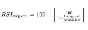
RSI
RSI (Relative Strength Index) is a technical analysis indicator that measures the momentum of a moving price. The indicator looks at the strength of the historical gains and losses, usually on a 14 day period. When the index is under 30, a stock is considered to be oversold. When the index is over 70, a stock is considered to be overbought. Taken from Investopedia, here is the formula for RSI:
MACD
MACD (Moving Average Convergence Divergence) is another technical analysis indicator that measures momentum. It tracks the relationship between two EMA (Exponential Moving Average), typically a 12-26 EMA of a stock, also called the MACD line, and the 9 EMA of the actual MACD line, called the signal line. When the MACD line crosses the signal line from under, this is said to be a buy signal. Conversely, when the MACD line crosses from above, it is a sell signal. Taken from Investopedia, here is the formula for the MACD line:

Let's make a new dataframe to calculate our indicators.
# Create new dataframe for indicators
indicators = coinmarketcap[['date', 'close']]
# Keep only observations from the last 2 years
indicators = indicators[indicators.date >= dt.date(2017, 8, 1)]
# Reset the index for consistency
indicators = indicators.reset_index(drop=True)
indicators.head()
Calculate the RSI for the price of bitcoin over a 14 day period. Start by calculating the change in closing prices for each row.
# Calculate the change in price from yesterday's close to today's close
change = []
for i, row in indicators.iterrows():
    x = row.close - indicators.loc[i-1, 'close'] if i > 0 else np.nan
    change.append(x)
indicators['change'] = change
indicators = indicators.dropna()
indicators = indicators.reset_index(drop=True)
indicators['upMove'] = [x if x >= 0 else 0 for x in indicators['change']]
indicators['downMove'] = [abs(x) if x < 0 else 0 for x in indicators['change']]
Now calculate the average upward movement over the last 14 days.
# Obtain an average of only upward price movements
avgUpMove = []
for i, row in indicators.iterrows():
    x = np.nan
    if i == 13:
        x = indicators[0:14]['upMove'].mean()
    elif i > 13:
        x = (avgUpMove[i-1] * 13 + row['upMove']) / 14
    avgUpMove.append(x)
indicators['avgUpMove'] = avgUpMove
Repeat the calculation with downward movement over the last 14 days.
# Obtain an average of only downward price movements
avgDownMove = []
for i, row in indicators.iterrows():
    x = np.nan
    if i == 13:
        x = indicators[0:14]['downMove'].mean()
    elif i > 13:
        x = (avgDownMove[i-1] * 13 + row['downMove']) / 14
    avgDownMove.append(x)
indicators['avgDownMove'] = avgDownMove
The RS or relative strength is the simply the average upward movement divided by the average downard movement. RSI is calculated by turning RS into an index. The formula is given below.
# Find the relative strength for the day
indicators['RS'] = indicators['avgUpMove'] / indicators['avgDownMove']
# Convert the relative strength to an index value (0-100 scale)
indicators['RSI'] = 100 - (100 / (indicators['RS'] + 1))
Calculate the 12-26-9 MACD indicator. We start by calculating the 12 day EMA.
# Calculate 12 day EMA
EMA12 = []
for i, row in indicators.iterrows():
    x = np.nan
    if i == 11:
        x = indicators[0:12]['close'].mean()
    elif i > 11:
        x = (row['close'] - EMA12[i-1]) * (2 / 13) + EMA12[i-1]
    EMA12.append(x)
indicators['EMA12'] = EMA12
Next, calculate the 26 day EMA.
# Calculate 26 day EMA
EMA26 = []
for i, row in indicators.iterrows():
    x = np.nan
    if i == 25:
        x = indicators[0:26]['close'].mean()
    elif i > 25:
        x = (row['close'] - EMA26[i-1]) * (2 / 27) + EMA26[i-1]
    EMA26.append(x)
indicators['EMA26'] = EMA26
The MACD line is simply the 26 day EMA subtracted by the 14 day EMA.
# Calculate MACD Line
indicators['MACD'] = indicators['EMA26'] - indicators['EMA12']
indicators = indicators.dropna()
indicators = indicators.reset_index(drop=True)
The signal line is the 9 day EMA of the MACD line.
# Calculate Signal Line (9 Day EMA for MACD Line)
signal = []
for i, row in indicators.iterrows():
    x = np.nan
    if i == 8:
        x = indicators[0:9]['MACD'].mean()
    elif i > 8:
        x = (row['MACD'] - signal[i-1]) * (2 / 10) + signal[i-1]
    signal.append(x)
indicators['signal'] = signal
We now have both of our indicators. Let's see how well these indicators work on BTC price data.
fig = plt.figure(figsize=(20, 12))
ax1 = fig.add_axes([0.1, 0.4, 0.8, 0.8])
ax2 = fig.add_axes([0.1, 0.1, 0.8, 0.3])

ax1.plot(indicators.date, indicators.close)
ax2.plot(indicators.date, indicators.RSI, 'r')

RSI_buy = indicators[indicators.RSI == indicators.RSI.min()]
RSI_buy
RSI_sell = indicators[(indicators.date > dt.date(2018, 11, 20)) & (indicators.RSI > 70)].iloc[0]
RSI_sell
RSI_gain = RSI_sell.close - RSI_buy.close
RSI_gain
If we bought BTC at its lowest level of RSI (indicating that BTC has been strongly oversold) and we sold BTC as soon as the RSI was greater than 70 (indicating a sell signal), we would have lost $504.78. Keep in mind that this is one test sample on the 14 day period only.
fig = plt.figure(figsize=(20, 12))
ax1 = fig.add_axes([0.1, 0.4, 0.8, 0.8])
ax2 = fig.add_axes([0.1, 0.1, 0.8, 0.3])

macd = ['MACD', 'signal']

ax1.plot(indicators.date, indicators.close)
for col in macd:
    ax2.plot(indicators.date, indicators[col])
ax2.legend(macd)

From performing visual analyzation the MACD line, if we bought around the very end of 2017 after the MACD crosses the signal line, we would have bought right after the peak of bitcoin and at the start of the bear market. Again, this only one observation, however this would have been a huge loss no matter what.
It seems that technical analysis might not be the best technique for analyzing price pattern or making price predictions. The crypto market is still young so this makes a lot of sense. The crypto market does not seem to follow patterns the way the stock market and forex market do. Let's see if we can use a linear model to predict the price of BTC.
Building A Predictive Model
We collected our data, cleaned the data for management, and visualized the data so we could better understand it. Now we will try and use the data to make a predictive model to make guesses on Bitcoin's price. The model we will use is linear regression, a simple form of machine learning. First we will test a model trained on active addresses data. Then we will test another model trained on transfer volume data. Finally we will test a model trained on both sets of data. My hypothesis is that bitcoin price data is more strongly correlated when using multiple linear regression. We will test this hypothesis by calculating R-squared values for each linear model.
Let's first train a model on active addresses.
# Obtain active addresses data and bitcoin price data
x_data = btc[['activeAddresses']]
y_data = btc.price

# Train the model on 75% of the data then test it on 25%
x_train, x_test, y_train, y_test = model_selection.train_test_split(x_data, y_data, test_size=.25)

# Train the model
model = LinearRegression()
model.fit(x_train, y_train)

# Obtain the coefficient
model.coef_
# Test the model on data it hasn't seen before
predicted = model.predict(x_test)

# Plot the results
fig, ax = plt.subplots(figsize=(20, 12))
plt.title('Linear Regression')
sns.distplot(y_test, hist=False, label="Actual", ax=ax)
sns.distplot(predicted, hist=False, label="Predicted", ax=ax);

model.score(x_test, y_test)
Now let's train a model on transfer volume.
# Obtain transfer volume data and bitcoin price data
x_data = btc[['transferVolume']]
y_data = btc.price

# Train the model on 75% of the data then test it on 25%
x_train, x_test, y_train, y_test = model_selection.train_test_split(x_data, y_data, test_size=.25)

# Train the model
model = LinearRegression()
model.fit(x_train, y_train)

# Obtain the coefficient
model.coef_
# Test the model on data it hasn't seen before
predicted = model.predict(x_test)

# Plot the results
fig, ax = plt.subplots(figsize=(20, 12))
plt.title('Linear Regression')
sns.distplot(y_test, hist=False, label="Actual", ax=ax)
sns.distplot(predicted, hist=False, label="Predicted", ax=ax);

model.score(x_test, y_test)
Finally, we'll train a model using multiple linear regression on both active addresses and transfer volume.
# Obtain transfer volume data and bitcoin price data
x_data = btc[['activeAddresses', 'transferVolume']]
y_data = btc.price

# Train the model on 75% of the data then test it on 25%
x_train, x_test, y_train, y_test = model_selection.train_test_split(x_data, y_data, test_size=.25)

# Train the model
model = LinearRegression()
model.fit(x_train, y_train)

# Obtain the coefficient
model.coef_
# Test the model on data it hasn't seen before
predicted = model.predict(x_test)

# Plot the results
fig, ax = plt.subplots(figsize=(20, 12))
plt.title('Linear Regression')
sns.distplot(y_test, hist=False, label="Actual", ax=ax)
sns.distplot(predicted, hist=False, label="Predicted", ax=ax);

model.score(x_test, y_test)
The R-squared value for a model trained only on the number of active addresses in the Bitcoin network was 0.574. This means that active addresses account for 57.4% of the variation in Bitcoin price. The R-squared value for a model trained only on the total USD value of transfer volume was 0.818. This means that transfer volume accounts for 81.1% and is more strongly correlated with Bitcoin price data. When we perform multiple linear regression, we get an R-squared value of 82.3% which suggests that this is a better predictive model.
Conclusion
The goal of this tutorial was to guide a reader through the data science life cycle while also sparking an interest in cryptocurrencies and blockchain technology. We learned how to Bitcoin price data from the internet and convert our data into dataframes. We took our cleaned data and used them to look at three case studies relating to cryptocurrencies. In the first case study we learned what the blockchain was and how different metrics of the blockchain are related to the overall price of a cryptocurrency. In the second case study we learned that Bitcoin remains the most dominant cryptocurrency in the crypto market, despite the it's skepticism. In the last case study we discovered that traditional technical analysis techniques do not work quite as well on cryptocurrencies since they are a newer market. Instead, we used linear regression, a form of machine learning to find the relationship between number of active Bitcoin addresses and total Bitcoin transfer volume against the price of Bitcoin. We discovered that by building a model using multiple linear regression, we can produce more accurate predictions.
The hope of this tutorial not for the reader to walk away feeling like they fully understand the topics introduced. It is the opposite. I hope that readers walk away with a newfound sense of curiousity for data science and blockchain technology. There were so many things we could have done differently in this project. We could have looked at different metrics, played with different currencies, even tried a more advanced machine learning model. Go out and try one of these in your own project!